
Freshwater Explorer Quick Guides
- Freshwater Explorer (Version 1.0) Quick Guide
- Freshwater Explorer (Version 2.0) Quick Guide
- List of Abbreviations
- Glossary
Access Freshwater Explorer (Version 1.0)
Access Freshwater Explorer (Version 2.0)
EPA's Freshwater Explorer is an interactive web-based mapping tool for water quality parameters of freshwater streams, lakes, and wells in all 50 U.S. states, Puerto Rico, and the U.S. Virgin Islands. This page contains Quick Guides with visual aids that explain how to use Freshwater Explorer, and a List of Abbreviations and Glossary of terms used within the tool.
EPA currently offers two versions of the Freshwater Explorer tool — Version 2.0 expands on Version 1.0's capabilities.
Please Note: Freshwater Explorer Version 1.0 will be retired in August 2025. Freshwater Explorer Version 2.0 will remain online in its place, offering enhanced functionality for users.
Freshwater Explorer (Version 1.0) Quick Guide
Overview
- EPA’s Freshwater Explorer works best when launched with Google Chrome.
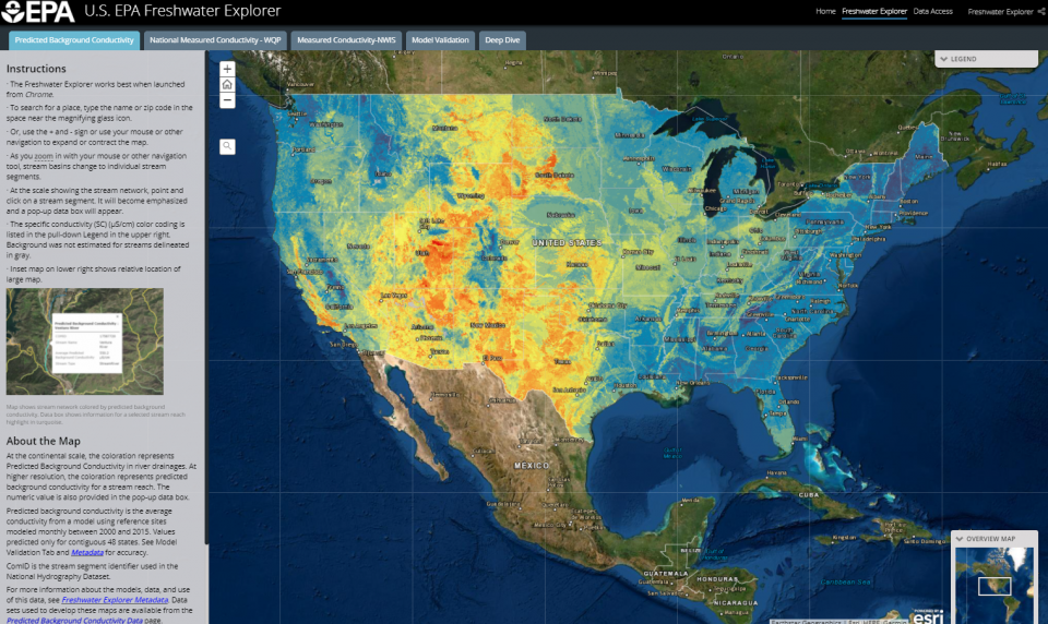
- On the landing page, scroll past the opening title until a colorful map of the United States appears. Wait for it to load.
Colors—Maps in Freshwater Explorer show predicted fresher water in blue, and more mineralized water in yellow.
Tabs allow you to explore pre-loaded searches or do your own deep dive. The first four tabs at the top are fixed views. It’s a good way to try the Explorer. Information about these views is in the pull-down menus on the left of each view. The fifth tab, “Deep Dive,” allows you to customize your view and pull in data from other publicly available web servers.
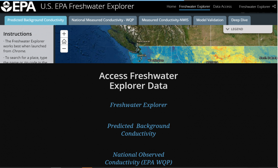
Data and metadata—Links are in the information at the top right “Data Access,” in pop-up boxes, or scroll down for the link list and disclaimer as shown here.
How to Search
- Expand or contract the map by using the + and - symbols or other navigation tools.
- Type the name or zip code in the space near the magnifying glass icon.
- As you zoom in with your mouse or other navigation tool, more detail and layer options become available, and the stream network becomes more complex.
- Point and click on a colored line or shape. A data box will appear with information about the location.
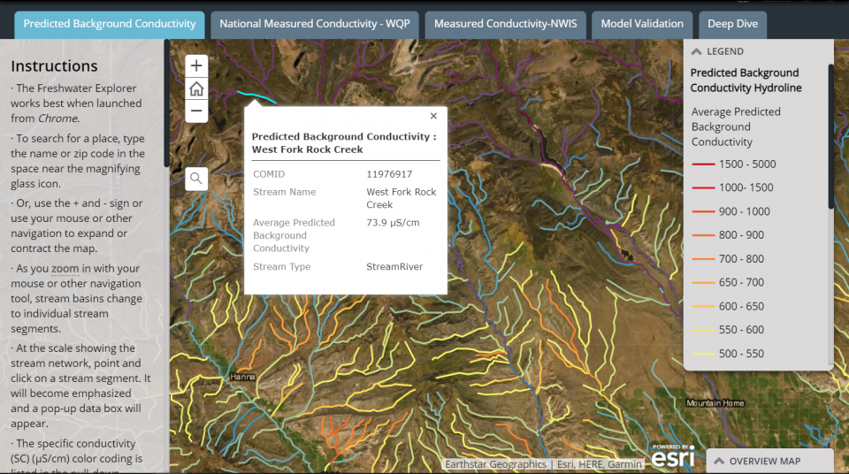
- The specific conductivity (SC; µS/cm) color coding is listed in the pull-down Legend in the upper right. Background was not estimated for streams delineated in gray. The inset map on the lower left shows the relative location of large map.
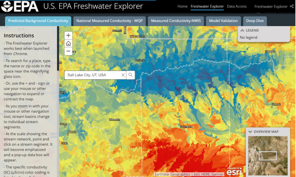
Predicted Background Conductivity—This is the first view when you open Freshwater Explorer. At the continental scale, colors represent predicted background conductivity in river drainages as they would occur if water quality was minimally disturbed by people. As you zoom in on an area, the background switches to satellite imagery showing vegetation and development. A network of streams appears as a spectrum from low (violet) to high (red) calculated natural background conductivity. Calculated dissolved mineral content is the average monthly conductivity modeled for 2000-2015. Click on a stream segment. It will become emphasized and a pop-up data box with predicted background conductivity will appear.
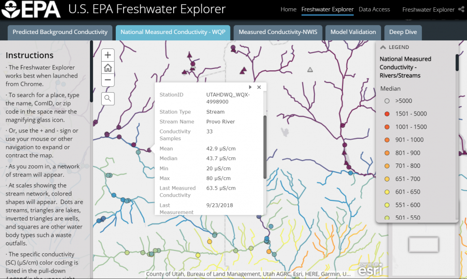
National Measured Conductivity-WQP—The second tab shows sample stations from WQX on a simple background with the stream network. Shapes are water body types listed in the legend on the right. Click on a station or a stream and a data box will appear. At the top of the box, numbers list the number of stations at this point. Use the triangle to see information from WQP or the stream segment background.
National Measured Conductivity– NWIS —The third tab shows sample stations from the National Water Information System (NWIS) on a simple background with the stream network. Shapes are water body types listed in the legend on the right. Click on a station or a stream segment and a data box will appear. At the top of the box, numbers list the number of stations at this point. Use the triangle to see information from WQP or the stream segment background.
Model Validation—This map shows how well the Predicted Background Conductivity (PBC) model performed by comparing conductivity measured at reference sites (dots) that were used to develop the empirical PBC model with the prediction from the model.

Deep Dive—Widgets in the upper right allow you to select background base maps, data layers such as measured data or predicted background, water body type, and pull in data from other public web services. The legends for each data layer are below the data layer you select.
Disclaimer: Some streams, especially headwaters, are not always captured in the NHDPlusV2 stream network. Observed data are from secondary sources. Use caution as some data have incorrect units (i.e. measured as mS/cm but entered as µS/cm, or vice versa, an error of 1000-fold). Data evaluation is a continuous process. Gray shapes indicate that the data has been flagged due to uncertain data quality.
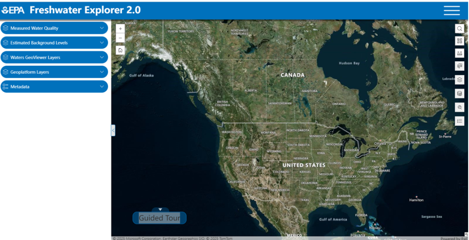
Freshwater Explorer (Version 2.0) Quick Guide
Overview
EPA’s Freshwater Explorer works best when launched with Google Chrome. The opening view shows a map of the United States.
- Zoom in or search for any location.
- Make a map by adding Freshwater Explorer data layers related to your area of interest.
- Access geospatial layers produced by other organizations to aid your discovery.
- Use tools or export data to analyze the information.
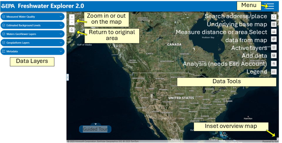
Navigation
- Data layers can be added to the map from the blue oblong dropdown buttons on the left.
- Tools appear as icons in white squares and can be used to interact and modify the map.
- The plus (+) and minus (-) signs allow the user to zoom in or out on the map.
- The Home icon allows the user to return to the original area.
- The three horizontal lines in the top right corner are the Menu.
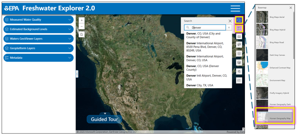
How to make a map
Step 1: Choose a place.
- Select the magnifying glass on the right.
- Type a name in the provided space. In our example, Denver, CO.
- For simplicity, choose a plain base map. In our example, we selected the Human Geography Map.
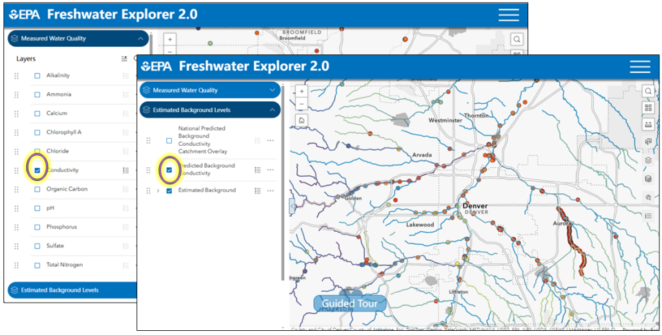
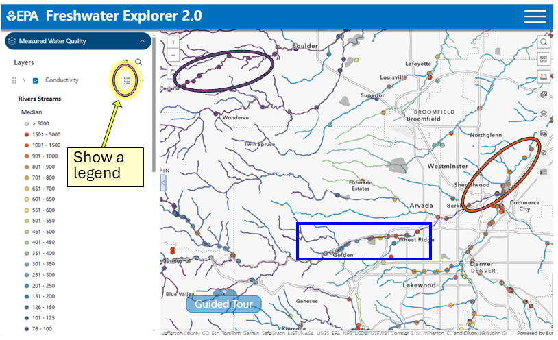
- Select "Conductivity" from the "Measured Water Quality" layer.
- Select "Predicted Background Conductivity" from the "Estimated Background Levels" layer.
- When the observed station value is the same color (shown in purple oval) as the stream background or regional 25th centile of geomeans of observed stations in an ecoregion, then anthropogenic inputs are less likely, compared to warm colors, such as orange on a cool-colored blue stream (shown in orange oval).
- To illustrate how it is easy to see anomalies: here, we selected a transition from blue to red stations on a purple stream (shown in blue rectangle).
- The horizontal lines next to the checked data layer in the left-hand menu shows the user a legend.
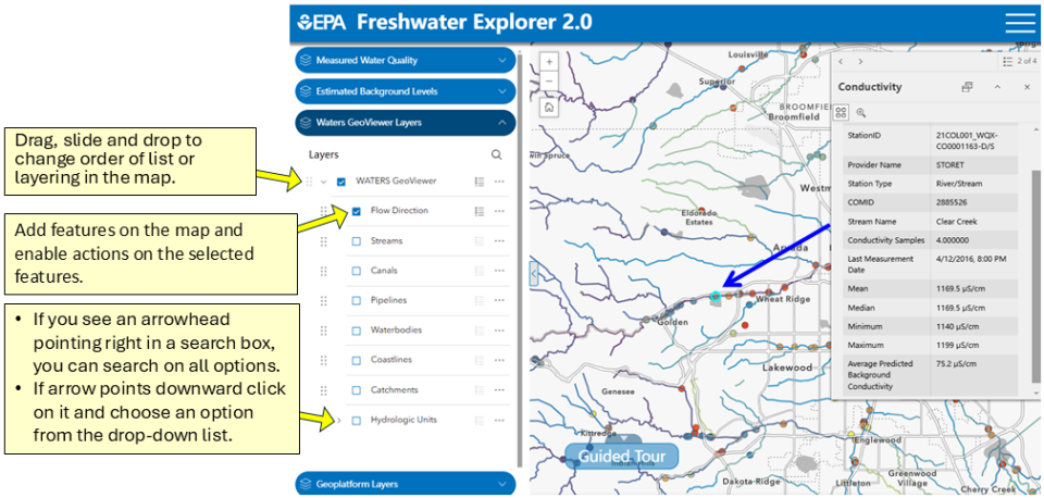
- The pop-up box shows that the measured value 1170 µS/cm is much greater than the average predicted background of 75 µS/cm.
- The user can drag, slide, and drop to change the order of the data layer list or the layering in the map by using the six dots to the left of the checked layer.
- Checking the box next to the layer name adds features on the map and enables actions on the selected feature.
- If you see an arrowhead pointing right in a search box, you can search on all options. If the arrowhead points downward, the user can click on it and choose an option from the drop down list.
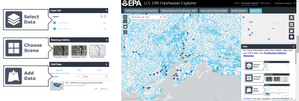
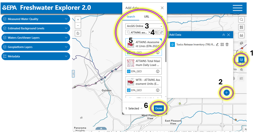
Step 2: Add data to learn more.
- Choose the add data icon.
- Select the plus sign.
- Type a search term in the search box (e.g., ATTAINS Assessment lines).
- Use the information icon for metadata on the layer.
- Choose the layer that you want.
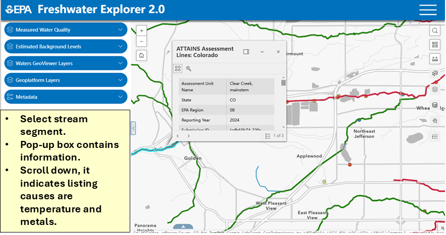
- Select Done and the data layer is added to the map shown in the following screenshot.
- Streams that obtain their designated uses are green and streams that do not are red.
- Selected stream segment is highlighted in a light blue color.
- Select the stream segment. The pop-up box will contain the stream information.
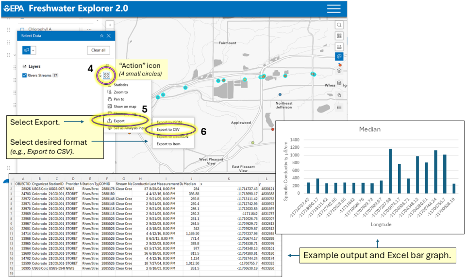
Step 3: Export data.
- Choose select data.
- Choose select by lasso.
- Outline the stations of interest with cursor, they will become highlighted in blue.
- Choose "Action" icon (4 small circles).

- Select Export.
- Select desired format (e.g., Export to CSV).
List of Abbreviations
| Term | Definition |
|---|---|
|
% Pleco |
Percentage of plecopteran taxa |
|
%Chiro |
Percentage of chronimid taxa |
|
%Cllct |
Percentage of collectors |
|
%Dip |
Percentage of dipteran taxa |
|
%Ephem |
Percentage of ephemeropteran taxa |
|
%EPT |
Percentage of ephemeropteran, plecopteran, and trichopteran taxa |
|
%Filtr |
Percentage of filterers |
|
%Oligo |
Percentage of oligochaete taxa |
|
%Pred |
Percentage of predators |
|
%Scrap |
Percentage of scrapers |
|
%Shred |
Percentage of shredders |
|
%Toler |
Percentage of tolerant taxa |
|
%Trich |
Percentage of trichopteran taxa |
|
B-C |
background-to-criterion |
|
CCC |
criterion continuous concentration |
|
CDF |
cumulative distribution function |
|
CI |
confidence interval |
|
CMEC |
criterion maximum exposure concentration |
|
DO |
dissolved oxygen |
|
EMAP |
Environmental Monitoring and Assessment Program |
|
EPA |
U.S. Environmental Protection Agency |
|
EPA |
Environmental Protection Agency |
|
GAM |
generalized additive model |
|
GIS |
Geographic Information System |
|
HCx |
hazardous concentration of the “x” centile of a taxonomic sensitivity distribution |
|
LOWESS |
Locally Weighted Scatterplot Smoothing |
|
MAHA |
Mid‑Atlantic Highland Assessment |
|
MAIA |
Mid‑Atlantic Integrated Assessment |
|
NAPAP |
National Acid Precipitation Assessment Program |
|
NRSA |
National Rivers and Streams Assessment |
|
NWSA |
National Wadeable Streams Assessment |
|
ORD |
Office of Research and Development |
|
ORD |
U.S. EPA Office of Research and Development |
|
OW |
U.S. EPA Office of Water |
|
OWOW |
U.S. EPA Office of Water Oceans and Wetlands |
|
PL |
prediction limit |
|
QA/QC |
quality assurance/quality control |
|
RBP |
rapid bioassessment protocol |
|
Region 6 |
U.S. EPA Region 6 |
|
R-EMAP |
Regional Environmental Monitoring and Assessment Program |
|
S |
Siemens |
|
SAB |
Science Advisory Board |
|
SC |
specific conductivity |
|
TDS |
total dissolved solids |
|
TMDL |
total maximum daily load |
|
TSS |
total suspended solids |
|
USGS |
U.S. Geological Survey |
|
WABbase |
Watershed Assessment Branch database |
|
WDE |
Washington Department of Ecology |
|
WoE |
Weight of Evidence |
|
WQP |
Water Quality Portal |
|
WQX |
Water Quality Exchange |
|
WSA |
Wadeable Streams Assessment |
|
WVDEP |
West Virginia Department of Environmental Protection |
|
XCD |
extirpation concentration distribution |
|
XCx |
extirpation concentration affecting “x” percentage of individuals of a taxon |
Glossary
| Term | Definition |
|---|---|
|
Anion |
A negatively charge ion, e.g., Cl- |
|
Assemblage, stream |
A taxonomic or sampled subset of a community as may be collected from a stream. |
|
Assessment endpoint |
An explicit expression of the actual environmental value that is to be protected, operationally defined by an ecological entity and its attribute or characteristics. An assessment endpoint may be identified at any level of organization (e.g., organism, population, community). |
|
Background |
The range of naturally occurring substances in waters that have not been substantially influenced by human activity. |
|
Background specific conductivity |
The specific conductivity (SC) in streams in a region that occurs naturally and not as the result of human activity. Background may also be characterized as a population of minimally affected sites or low SC sites using a weight of evidence. |
|
Background-to-Criterion (B-C) Model |
A log-log linear regression model of the background conductivity values associated with the estimated 5% extirpation of stream organisms from 24 ecoregions in the United States (Cormier et al 2018). |
|
Benchmark |
A dose or concentration of a pollutant that, if exceeded, is expected to produce an adverse effect (called the benchmark response) in one or more assessment endpoints, signifying a decline in water quality or human health. |
|
Bootstrapping |
A statistical technique of repeated random sampling from a data set that is often used in environmental studies to estimate confidence and prediction limits of a parameter. |
|
Box plot |
A depiction of the 25th, 50th, and 75th quantiles of a distribution as a rectangle with a central line. The two standard deviation range is depicted as “whiskers” extending from the box. Data beyond two standard deviations are indicated by individual circles or dots beyond the whiskers. |
|
Catchment area |
The spatial extent of the surrounding landscape that drains into a particular river, stream, or other waterbody. |
|
Cation |
A positively charged ion, e.g., Na+ |
|
Community |
The full complement of interacting organisms within a defined area of an ecosystem. |
|
Conductance, specific |
Conductance is the inverse of resistance for a particular sample expressed as Seimens (S) usually at 25°C. In the literature, it is sometimes used synonymously with specific conductivity, but to avoid confusion, the term conductance is not used in this document. |
|
Conductivity, specific (or specific electrical conductivity) |
A measure of ionic concentration based on the electrical property of water and dissolved ions. As ionic concentration increases, conductivity increases. Standardized measurements in this document refer to specific conductivity, μS/cm (also seen as: μmho/cm) at 25°C. |
|
Confounder |
An extraneous variable that correlates with both the dependent and independent variable. The presence of confounders can interfere with the ability to characterize a causal relationship. |
|
Criterion continuous concentration (CCC) |
An estimate of the highest concentration of a material in surface water to which an aquatic community can be exposed indefinitely without resulting in an unacceptable effect. |
|
Criterion maximum exposure concentration (CMEC) |
An estimate of the maximum concentration of a material in surface water to which an aquatic community can be exposed for a short time without resulting in an unacceptable effect. In this document, the CMEC is estimated at the 90th centile of specific conductivity observations that contribute to the annual CCC. |
|
Cumulative frequency distribution (CFD) |
The probabilities that a random variable with a given probability distribution will be found at a value less than or equal to x. Weighted CFDs are used to estimate extirpation concentrations of individual genera or species and unweighted CFDs to estimate a SC level that is expected to extirpate 5% of aquatic invertebrate genera. Similar to cumulative distribution function (CDF) |
|
Ephemeral stream |
A stream that flows briefly only in direct response to local precipitation, and whose channel is above the local ground water table at all times. |
|
Extirpation |
The depletion of a population of a species or genus to the point that it is no longer a viable resource or is unlikely to fulfill its function in the ecosystem. |
|
Extirpation concentration |
The level above which a genus is effectively absent from its normal habitat. The threshold for extirpation is operationally defined by the level below which 95% of the observations of the genus occur. |
|
Extrapolation |
The process of extending the applicability of a model beyond the measured range of the original data set from which the model was derived. |
|
Flowing waters |
Inland waters with a unidirectional flow including permanent, intermittent and ephemeral streams. |
|
Fresh water |
Naturally occurring water characterized by low concentrations of dissolved salts and other total dissolved solids, not brackish or marine water. |
|
Freshwater |
Adjective indicating low salt content, typically less than 1,000 ppm or 1500uS/cm. |
|
Generalized additive model |
A nonparametric, likelihood based local regression model that replaces the linear function of a generalized linear model with a locally smoothed additive function. |
|
Hazardous concentration |
A concentration threshold that is hazardous for a proportion of taxa. In this document, it is the concentration that is hazardous to 5% of genera calculated as the 5th centile of a taxonomic extirpation concentration distribution. |
|
Hydroline |
A feature-based database that interconnects and uniquely identifies the stream segments or reaches that make up the nation's surface water drainage system. The National Hydrography Dataset (NHD) data was originally developed at 1:100,000-scale and exists at that scale for the whole country. |
|
Hydrology |
Distribution and connectivity of water such as streams and lakes |
|
Intermittent stream |
A stream that flows continuously for only part of the time. During low flow there may be dry reaches alternating with wetted, nonflowing reaches. The stream bed may lie below the local ground water table for at least part of the year. |
|
Interpolate |
Process of estimating an unknown value that lies between known values. |
|
Ion |
an atom or molecule with a net electric charge due to the loss or gain of one or more electrons, e.g., Na+ or Cl- |
|
Ionic composition |
The specific ions dissolved in water. In this document, the ionic composition is used to distinguish water dominated by chloride salts from those dominated by bicarbonate and sulfate salts. |
|
Ionic mixture |
An undefined or defined blend of dissolved ions. In this document, the example case studies refer to the most common mixture of ions contaminating U.S. streams, specifically those dominated by calcium, magnesium, sulfate, and bicarbonate ions. |
|
Ionic regulation |
The passive and active physiological processes that maintain the ionic composition, pH, and water content of tissues that is necessary for life. |
|
Least disturbed condition |
The best available physical, chemical, and biological habitat conditions given today’s state of the landscape or the least disturbed by human activities (Stoddard et al., 2006). Contrast with “minimally affected condition.” |
|
Major ions |
The most common contributors to ionic concentration in surface waters, consisting of the following cations: Ca2+, Mg2+, Na+, K+; and anions: HCO3−, CO32−, SO42−, Cl−. |
|
Measure of effect |
A measurable ecological characteristic that is related to the valued characteristic chosen as the assessment endpoint and is a measure of biological effects (e.g., survival, reproduction, growth). In this document it is the presence/absence of macroinvertebrate genera along a specific conductivity gradient. |
|
Measure of exposure |
An observed or estimated characteristic that is used to characterize the level of exposure to the stressor. In this document, the measure of ionic exposure is specific conductivity. |
|
Minimally affected condition |
The physical, chemical, and biological habitat found in the absence of significant human disturbance (Stoddard et al., 2006). Contrast with “least disturbed condition.” |
|
Osmoregulation |
The physiological control of water content of an organism's tissues to maintain fluid and electrolyte balance within a cell or organism relative to the surrounding environment. |
|
Perennial stream |
A stream with continuous surface or shallow interstitial flow year round, and whose stream bed intersects the local ground water table throughout the year. Also referred to as a permanent stream. |
|
Predicted 5% Extirpation Concentration |
The concentration that is hazardous to 5% of genera calculated as the 5th centile of a taxonomic extirpation concentration distribution. |
|
Predictive background conductivity |
Mineral content is the average conductivity predicted monthly for years 2000 – 2015 as they would occur if water quality was minimally influenced by people. |
|
Predictive background conductivity model |
A random forest regression model that predicts background conductivity based on geophysical and other data at thousands of sites that were judged to be relatively unaffected by people (Olson and Cormier 2019). |
|
Produced water |
Waters that are produced by oil and gas development, mine dewatering, and related activities (e.g., coal bed methane mining, hydraulic fracturing). |
|
Reference site |
Sampling locations that have been identified as minimally affected or least disturbed based on land use, habitat, and water quality characteristics other than specific conductivity. |
|
Salinity |
The amount of salts dissolved in water. Traditionally expressed as parts per thousand (‰) or grams of salt per kilogram of water. Salinity (‰) is often reserved for describing marine waters where sodium and chloride are the dominant ions. In this report, salinity is equivalent to total dissolved salts and may be composed of any ionic mixture. |
|
Sample |
A single water or biological collection, multiple samples can be taken at different times. |
|
Sample site |
Location where a water or biological collection was taken. |
|
Sensitivity analysis |
A process that involves changing input values of a model in various ways to see the effect on the output value. The main goal of sensitivity analysis is to gain insight into which assumptions are most critical for model building. |
|
Station |
Location where a water or biological collection was taken. |
|
Topography |
Mapped forms and features of land surfaces. |
|
Total dissolved solids (TDS) |
A measure of the combined content of all inorganic and organic substances dissolved in water, conventionally expressed as mg/L and operationally defined as those solids that pass through a filter, typically 0.45 μm. |
|
Total Nitrogen |
Sum of nitrate+nitrite and total Kjeldahl nitrogen (TKN) in mg/L. |
|
Total Phosphorus |
Data reported as phosphorus were converted to standardized forms and where appropriate summed as Total Phosphorus, Dissolved Phosphorus, Total Orthophosphate, Dissolved Orthophosphate. |
|
Univoltine |
An organism having one brood or generation per year. |
|
Validation |
Confirmation of the quality of a model and its results, typically by applying an independent data set. |
|
Valley fill |
A headwater valley filled with mining overburden. This practice usually occurs in steep terrain where there are limited disposal alternatives. |
|
Verification |
Demonstrating the accuracy of measurements or calculations. |
|
Weight of Evidence |
(1) A process of making inferences from multiple pieces of evidence, adapted from the legal metaphor of the scales of justice. (2) The relative degree of support for a conclusion provided by evidence. The result of “weighing the body of evidence.” |
|
Wells |
May refer to freshwater wells or oil and gas wells. |
|
Widget |
A tool or subroutine used in the U.S. EPA Freshwater Explorer. |